Bayesian analysis of longitudinal multilevel data using brms and rethinking - part 2

Part 2 of a tutorial showing how to fit Bayesian models using the rethinking package.

Author

Andreas Handel

Published

February 23, 2022

This is part two of a tutorial illustrating how to perform a Bayesian analysis of longitudinal data using a multilevel/hierarchical/mixed-effects setup. In this part, we’ll fit the simulated data using the rethinking package.

I assume you’ve read part 1, otherwise this post won’t make much sense. You might even want to open that first part in a separate tab for quick comparison.

Introduction

In the previous post, I showed a setup where some continuous outcome data (in our case, virus load) was collected over time for several individuals. Those individuals differed by some characteristic (in our case, dose at which they got infected). I specified several models that are useful for both fitting the data, and creating simulations. We’ve done the simulating part, now we’ll start fitting models to that data.

The advantage of fitting to simulated data is that we know exactly what model and what parameters produced the data, so we can compare our model estimates to the truth (i.e. the parameter and model settings that were used to generate the data) to see how our models perform. It is always good to do that to get some confidence that your models make sense, before you apply them to real data. For the latter, you don’t know what the “truth” is, so you have to trust whatever your model tells you.

Fitting Bayesian models can take a good bit of time (hours, depending on the settings for the fitting routine). It is generally advisable to place code that takes a while to run into its own R script, run that script and then save the results for further processing. This is in fact what I did here. I wrote 2 separate R scripts, one that does the fitting and one that does the exploration of the model fits. The code shown below comes from those 2 scripts. There is some value in re-coding yourself by copying and pasting the code chunks from this tutorial, but if you just want to get all the code from this post you can find it here and here.

R Setup

We’ll start with loading needed packages. Make sure these packages are installed. Since rethinking uses the Stan Bayesian modeling engine, you need to install it too. It is in my experience mostly seamless, but at times it seems to be tricky. I generally follow the instructions on the rethinking website and it has so far always worked for me. It might need some fiddling, but you should be able to get them all to work.

library('dplyr') # for data manipulation
library('ggplot2') # for plotting
library('cmdstanr') #for model fitting
library('rethinking') #for model fitting
library('fs') #for file path

Data loading

We’ll jump right in and load the data we generated in the previous tutorial. In this example, I’m fitting the data that was generated by model 3 since it shows the most realistic pattern. You can try to fit to the other 2 datasets and see what you find (I’ll show an example in this part of the tutorial. It is not necessarily the case that the model that produced a certain dataset is also the one that fits it best.

# adjust as necessary
simdatloc <- here::here('posts','2022-02-22-longitudinal-multilevel-bayes-1','simdat.Rds')
simdat <- readRDS(simdatloc)
#using dataset 3 for fitting
#also removing anything in the dataframe that's not used for fitting
#makes the ulam/Stan code more robust
fitdat=list(id=simdat[[3]]$id,
            outcome = simdat[[3]]$outcome,
            dose_adj = simdat[[3]]$dose_adj,
            time = simdat[[3]]$time)
#pulling out number of observations
Nind = length(unique(simdat$m3$id))

Fitting with rethinking

We’ll start by fitting the different models we discussed in part 1 using the rethinking package. The main function in that package, which does the fitting using Stan, is ulam.

First, we’ll specify each model, then we’ll run them all in a single loop.

Model 1

These lines of code specify the full set of equations for our model 1. Note how closely the R code resembles the mathematical notation. That close match between math and code is one of the nice features of rethinking/ulam. Also note the indexing of the parameters a0 and b0 by id, which indicates that each individual has their own values.

#wide-prior, no-pooling model
#separate intercept for each individual/id
#2x(N+1)+1 parameters
m1 <- alist(
  # distribution of outcome
  outcome ~ dnorm(mu, sigma),

  # main equation for time-series trajectory
  mu <- exp(alpha)*log(time) - exp(beta)*time,

  #equations for alpha and beta
  alpha <-  a0[id] + a1*dose_adj,
  beta <-  b0[id] + b1*dose_adj,

  #priors
  a0[id] ~ dnorm(2,  10),
  b0[id] ~ dnorm(0.5, 10),

  a1 ~ dnorm(0.3, 1),
  b1 ~ dnorm(-0.3, 1),
  sigma ~ cauchy(0,1)
)

You might have noticed that I chose some of the values in the priors to be different than the values we used to generate the simulated data. I don’t want to make things too easy for the fitting routine 😁. We want to have the fitting routine “find” the right answer (parameter estimates). Hopefully, even if we don’t start at the right values, we’ll end up there.

Model 2

Now we’ll set up model 2 exactly as for model 1 but with some of the priors changed as discussed previously. Specifically, the priors now force the individual-level parameters to be essentially all the same. Note that - as you will see below - this model is not a good model, and if one wanted to not allow the $a_{0}$ and $b_{0}$ parameters to have any individual level variation, one should just implement and run the model 2 alternative I describe below. We’ll run this model anyway, to just illustration and to see what happens.

#narrow-prior, full-pooling model
#2x(N+2)+1 parameters
m2 <- alist(
  outcome ~ dnorm(mu, sigma),
  mu <- exp(alpha)*log(time) - exp(beta)*time,
  alpha <-  a0[id] + a1*dose_adj,
  beta <-  b0[id] + b1*dose_adj,
  a0[id] ~ dnorm(mu_a,  0.0001),
  b0[id] ~ dnorm(mu_b, 0.0001),
  mu_a ~ dnorm(2, 1),
  mu_b ~ dnorm(0.5, 1),
  a1 ~ dnorm(0.3, 1),
  b1 ~ dnorm(-0.3, 1),
  sigma ~ cauchy(0,1)
)

Model 3

This is the same as model 1 but with different values for the priors. These priors are somewhat regularizing and more reasonable. As we’ll see, the results are similar to those from model 1, but the model runs more efficiently and thus faster.

#regularizing prior, partial-pooling model
m3 <- alist(
  outcome ~ dnorm(mu, sigma),
  mu <- exp(alpha)*log(time) - exp(beta)*time,
  alpha <-  a0[id] + a1*dose_adj,
  beta <-  b0[id] + b1*dose_adj,
  a0[id] ~ dnorm(2,  1),
  b0[id] ~ dnorm(0.5, 1),
  a1 ~ dnorm(0.3, 1),
  b1 ~ dnorm(-0.3, 1),
  sigma ~ cauchy(0,1)
)

Model 4

This is our adaptive pooling model. For this model, we specify a few extra distributions.

#adaptive priors, partial-pooling model
#2x(N+2)+1 parameters
m4 <- alist(
  outcome ~ dnorm(mu, sigma),
  mu <- exp(alpha)*log(time) - exp(beta)*time,
  alpha <-  a0[id] + a1*dose_adj,
  beta <-  b0[id] + b1*dose_adj,
  a0[id] ~ dnorm(mu_a,  sigma_a),
  b0[id] ~ dnorm(mu_b, sigma_b),
  mu_a ~ dnorm(2, 1),
  mu_b ~ dnorm(0.5, 1),
  sigma_a ~ cauchy(0, 1),
  sigma_b ~ cauchy(0, 1),
  a1 ~ dnorm(0.3, 1),
  b1 ~ dnorm(-0.3, 1),
  sigma ~ cauchy(0, 1)
)

A few model alternatives

There are a few model alternatives I also want to consider. The first one is a version of model 2 that gets rid of individual-level parameters and instead has only population-level parameters. I discussed this model in part 1 of the tutorial and called it 2a there. Here is the model definition

Model 2a

#full-pooling model, population-level parameters only
#2+2+1 parameters
m2a <- alist(
  outcome ~ dnorm(mu, sigma),
  mu <- exp(alpha)*log(time) - exp(beta)*time,
  alpha <-  a0 + a1*dose_adj,
  beta <-  b0 + b1*dose_adj,
  a0 ~ dnorm(2,  0.1),
  b0 ~ dnorm(0.5, 0.1),
  a1 ~ dnorm(0.3, 1),
  b1 ~ dnorm(-0.3, 1),
  sigma ~ cauchy(0,1)
)

Note that a0 and b0 are not indexed by id anymore and are now single numbers, instead of $N$ values as before.

Model 4a

Another model I want to look at is a variant of model 4. This is in fact the same model as model 4, but written in a different way. A potential problem with model 4 and similar models is that parameters inside parameters can lead to inefficient or unreliable numerical results when running your Monte Carlo routine (in our case, this is Stan-powered Hamilton Monte Carlo). It is possible to rewrite the model such that it is the same model, but it looks different in a way that makes the numerics often run better. It turns out for our example, model 4 above runs ok. But it’s a good idea to be aware of the fact that one can re-write models if needed, therefore I decided to include this model alternative here.

The above model 4 is called a centered model and the re-write for model 4a is called a non-centered model. The trick is to pull out the parameters from inside the distributions for $a_{0, i}$ and $b_{0, i}$ . The non-centered model looks like this:

#adaptive priors, partial-pooling model
#non-centered
m4a <- alist(
  outcome ~ dnorm(mu, sigma),
  mu <- exp(alpha)*log(time) - exp(beta)*time,
  #rewritten to non-centered
  alpha <-  mu_a + az[id]*sigma_a + a1*dose_adj,
  beta  <-  mu_b + bz[id]*sigma_b + b1*dose_adj,
  #rewritten to non-centered
  az[id] ~ dnorm(0, 1),
  bz[id] ~ dnorm(0, 1),
  mu_a ~ dnorm(2, 1),
  mu_b ~ dnorm(0.5, 1),
  sigma_a ~ cauchy(0, 1),
  sigma_b ~ cauchy(0, 1),
  a1 ~ dnorm(0.3, 1),
  b1 ~ dnorm(-0.3, 1),
  sigma ~ cauchy(0, 1)

  )

Again, this model is mathematically the same as the original model 4. If this is confusing and doesn’t make sense (it sure wouldn’t to me if I just saw that for the first time 😁), check the Statistical Rethinking book. (And no, I do not get a commission for continuing to point you to the book, and I wish there was a free online version (or a cheap paperback). But it is a great book and if you want to learn this kind of modeling for real, I think it’s worth the investment.)

Model 5

Another model, which I’m calling model 5 here, is one that does not include the dose effect. That means, parameters $a_{1}$ and $b_{1}$ are gone. Otherwise I’m following the setup of model 1. The reason I’m doing this is because on initial fitting of the above models, I could not obtain estimates for the dose parameters I used for the simulation. I noticed strong correlations between posterior distributions of the model parameters. I suspected an issue with non-identifiable parameters (i.e, trying to estimate more parameters than the data supports). To figure out what was going on, I wanted to see how a model without the dose component would perform. It turned out that the main reason things didn’t look right was because I had a typo in the code that generated the data, so what I thought was the generating model actually wasn’t 🤦. A helpful colleague and reader pointed this out. Once I fixed it, things made more sense. But I figured it’s instructive to keep this model anyway.

#no dose effect
#separate intercept for each individual/id
#2xN+1 parameters
m5 <- alist(
  # distribution of outcome
  outcome ~ dnorm(mu, sigma),

  # main equation for time-series trajectory
  mu <- exp(alpha)*log(time) - exp(beta)*time,

  #equations for alpha and beta
  alpha <-  a0[id],
  beta <-  b0[id],

  #priors
  a0[id] ~ dnorm(2,  10),
  b0[id] ~ dnorm(0.5, 10),

  sigma ~ cauchy(0,1)
)

Setting starting values

Any fitting routine needs to start with some parameter values and then from there tries to improve. Stan uses a heuristic way of picking some starting values. Often that works, sometimes it fails initially but then the routine fixes itself, and sometimes it fails all the way. In either case, I find it a good idea to specify starting values, even if they are not strictly needed. And it’s good to know that this is possible and how to do it, just in case you need it at some point. Setting starting values gives you more control, and you also know exactly what should happen when you look at for instance the traceplots of the chains.

## Setting starting values
#starting values for model 1
startm1 = list(a0 = rep(2,Nind), b0 = rep(0.5,Nind), a1 = 0.3 , b1 = -0.3, sigma = 1)
#starting values for model 2
startm2 = list(a0 = rep(2,Nind), b0 = rep(0.5,Nind), mu_a = 2, mu_b = 1, a1 = 0.3 , b1 = -0.3, sigma = 1)
#starting values for model 3
startm3 = startm1
#starting values for models 4 and 4a
startm4 = list(mu_a = 2, sigma_a = 1, mu_b = 1, sigma_b = 1, a1 = 0.3 , b1 = -0.3, sigma = 1)
startm4a = startm4
#starting values for model 2a
startm2a = list(a0 = 2, b0 = 0.5, a1 = 0.3, b1 = -0.3, sigma = 1)
#starting values for model 5
startm5 = list(a0 = rep(2,Nind), b0 = rep(0.5,Nind), sigma = 1)

#put different starting values in list
#need to be in same order as models below
startlist = list(startm1,startm2,startm3,startm4,startm2a,startm4,startm5)

Note that we only specify values for the parameters that are directly estimated. Parameters that are built from other parameters (e.g. $α$ and $β$ ) are computed and don’t need starting values.

For some more detailed discussion on starting values, see for instance this post by Solomon Kurz. He uses brms in his example, but the same idea applies with any package/fitting routine. He also explains that it is a good idea to set different starting values for each chain. I am not sure if/how this could be done with rethinking, it seems ulam does not support this? But it can be done for brms (and I’m doing it there).

Model fitting

Now that we specified all models, we can loop through all models and fit them. First, some setup before the actual fitting loop.

#general settings for fitting
#you might want to adjust based on your computer
warmup = 3000 
iter = 5000
max_td = 15 #tree depth
adapt_delta = 0.999
chains = 5
cores  = chains
seed = 4321
# for quick testing, use the settings below
# results won't make much sense, but can make sure the code runs
#warmup = 600 #for testing
#iter = warmup + floor(warmup/2)
#max_td = 10 #tree depth
#adapt_delta = 0.99


#stick all models into a list
modellist = list(m1=m1,m2=m2,m3=m3,m4=m4,m2a=m2a,m4a=m4a,m5=m5)
# set up a list in which we'll store our results
fl = vector(mode = "list", length = length(modellist))


#setting for parameter constraints
constraints = list(sigma="lower=0",sigma_a="lower=0",sigma_b="lower=0")

The first code block defines various settings for the ulam function. Look at the help file for details. Then we place all models into a list, set up an empty list for our fit results, and specify the data needed for fitting. The final command enforces some constraints on parameters. For our model, we want Half-Cauchy distributions for all variance parameters to ensure they are positive. Above, I specified them as Cauchy. There is no direct Half-Cauchy implementation. The way one achieves one is to tell ulam/Stan that the values for those parameters need to be positive. That’s what the constraints line in the code below does.

Looping over each model and fitting it. In addition to the actual fitting call to ulam, I’m also printing a few messages and storing the model name and the time it took to run. That’s useful for diagnostic. It’s generally a good idea to do short runs/chains until things work, then do a large run to get the actual result. Recording the running time helps decide how long a real run can be and how long it might take.

# fitting models
#loop over all models and fit them using ulam
for (n in 1:length(modellist))
{

  cat('************** \n')
  cat('starting model', names(modellist[n]), '\n')

  tstart=proc.time(); #capture current time

  #run model fit
  fit <- ulam(flist = modellist[[n]],
                          data = fitdat,
                          start=startlist[[n]],
                          constraints=constraints,
                          log_lik=TRUE, cmdstan=TRUE,
                          control=list(adapt_delta=adapt_delta,
                                       max_treedepth = max_td),
                          chains=chains, cores = cores,
                          warmup = warmup, iter = iter,
                          seed = seed
  )# end ulam

  # save fit object to list
  fl[[n]]$fit <- fit
  
  #capture time taken for fit
  tdiff=proc.time()-tstart;
  runtime_minutes=tdiff[[3]]/60;

  cat('model fit took this many minutes:', runtime_minutes, '\n')
  cat('************** \n')

  #add some more things to the fit object
  fl[[n]]$runtime = runtime_minutes
  fl[[n]]$model = names(modellist)[n]

} #end fitting of all models

# saving the list of results so we can use them later
# the file is too large for standard Git/GitHub
# Git Large File Storage should be able to handle it
# I'm using a simple hack so I don't have to set up Git LFS
# I am saving these large file to a folder that is synced with Dropbox
# adjust accordingly for your setup
#filepath = fs::path("C:","Data","Dropbox","datafiles","longitudinalbayes","ulamfits", ext="Rds")
filepath = fs::path("D:","Dropbox","datafiles","longitudinalbayes","ulamfits", ext="Rds")
saveRDS(fl,filepath)

Explore model fits

Now we are ready to explore the model fitting results. All fits are in the list called fl. For each model the actual fit is in fit, the model name in model and the run time in runtime. Note that the code chunks below come from this second R script, thus some things are repeated (e.g., loading of simulated data).¹

# loading list of previously saved fits.
# useful if we don't want to re-fit
# every time we want to explore the results.
# since the file is too large for GitHub
# it is stored in a local folder
# adjust accordingly for your setup
filepath = fs::path("D:","Dropbox","datafiles","longitudinalbayes","ulamfits", ext="Rds")
if (!fs::file_exists(filepath))
{
  filepath = fs::path("C:","Data","Dropbox","datafiles","longitudinalbayes","ulamfits", ext="Rds")
}

fl <- readRDS(filepath)
# also load data file used for fitting
simdatloc <- here::here('posts','2022-02-22-longitudinal-multilevel-bayes-1','simdat.Rds')
simdat <- readRDS(simdatloc)
#pull the data set we used for fitting
#if you fit a different one of the simulated datasets, change accordingly
fitdat <- simdat$m3
#contains parameters used for fitting
pars <- simdat$m3pars

You should explore your model fits carefully. Look at the trace-plots or trank-plots with the traceplot() and trankplot() functions in rethinking. Make sure the chains are looking ok. You can also use the summary function to get some useful information on our model. To go further, you can call stancode() to get the actual Stan code for the model. This can be helpful to both learn Stan, and to check if the model translates into Stan code the way you expected it to.

I’m showing a few of those explorations to illustrate what I mean. For any real fitting, it is important to carefully look at all the output and make sure everything worked as expected and makes sense.

To keep output manageable, I’m using model 2a here, which has no individual-level parameters, thus only a total of 5.

# Model 2a summary
#show(fl[[5]]$fit)

# Model 2a trace plots
# for some reason didn't work on last compile
#rethinking::traceplot(fl[[5]]$fit, pars = c("a0","b0","a1","b1","sigma"))

# Model 2a pair plot
# Correlation between posterior samples of parameters
rethinking::pairs(fl[[5]]$fit, pars = c("a0","b0","a1","b1","sigma"))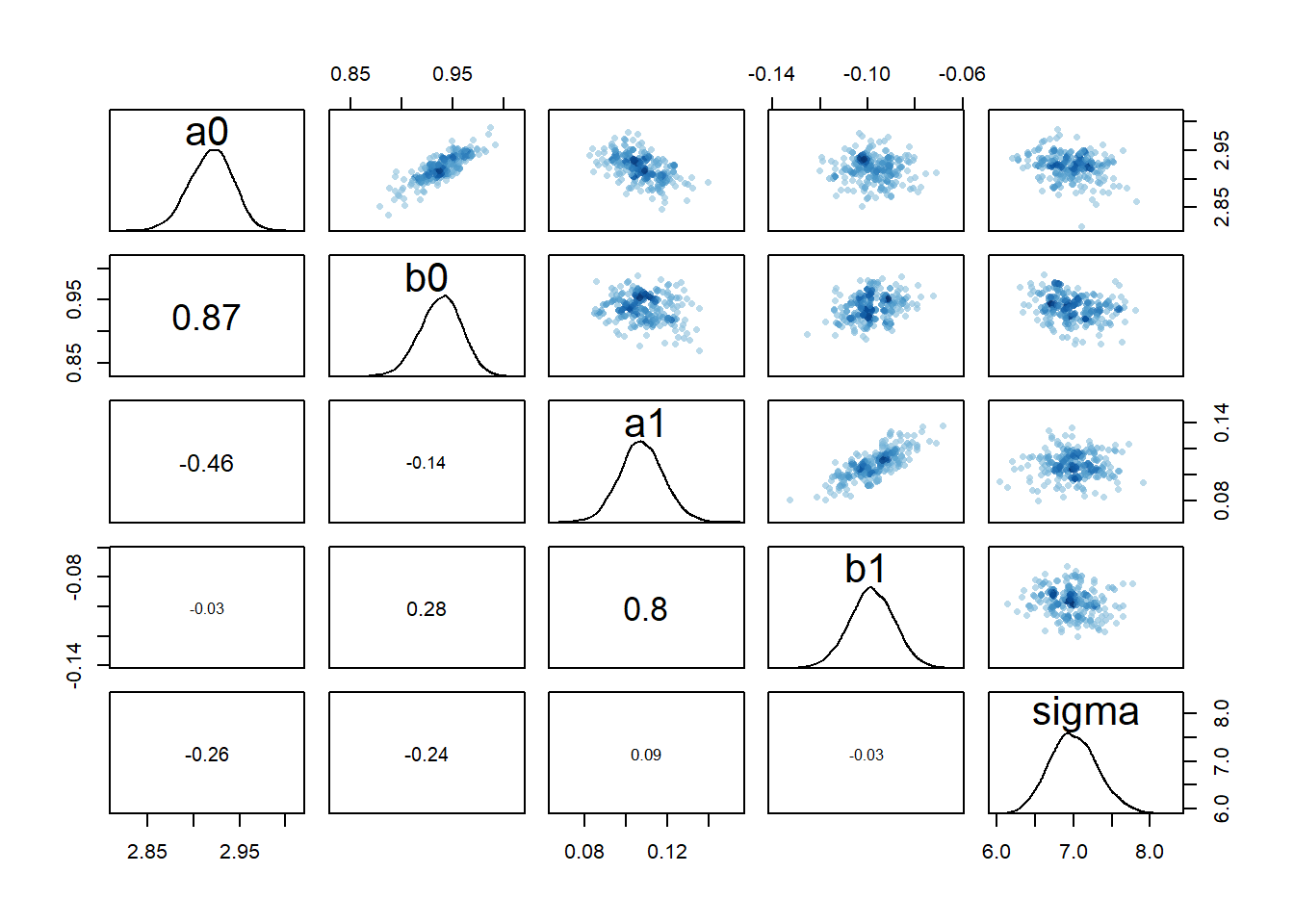

Based on these diagnostic outputs, it seems the chains converged well, at least for model 2a. One interesting feature is the strong correlation between the parameters $a_{0}$ and $b_{0}$ and also $a_{1}$ and $b_{1}$ . Recall that $α$ determined the initial increase of the function, $β$ the eventual decline. Both parameters determine the shape of the deterministic trajectory for all times, so large values for both can lead to somewhat similar results as small values for both. That is the reason for the correlations we see (and this is a different effect from the correlations we’ll discuss below).

Models 1 and 3

Now I’ll look at bit more carefully at the different models. We start by comparing fits for models 1 and 3. Those two are essentially the same model, with the only difference being wider priors for the individual-level parameters in model 1. It is worth mentioning that when running the fitting routine, model 1 takes much longer to fit than model 3. With the settings I used, runtimes were 214 versus 53 minutes. The wide priors made the fitting efficiency poor. But let’s see how it impacts the results.

First, we explore priors and posteriors. They are easy to extract from the models using the extract.prior() and extract.samples() functions from rethinking.

#get priors and posteriors for models 1 and 3
m1prior <- rethinking::extract.prior(fl[[1]]$fit, n = 1e4)
m1post <- rethinking::extract.samples(fl[[1]]$fit, n = 1e4)

m3prior <- rethinking::extract.prior(fl[[3]]$fit, n = 1e4)
m3post <- rethinking::extract.samples(fl[[3]]$fit, n = 1e4)

Now we can plot the distributions. Note that for the individual-level parameters $a_{0}$ and $b_{0}$ , the plots show the distribution across all individuals. The dashed lines show the priors, the solid the posteriors. Black is model 1, blue is model 3.

#showing density plots for a0
plot(density(m1prior$a0), xlim = c (-20,20), ylim = c(0,2), lty=2)
lines(density(m1post$a0), lty=1)
lines(density(m3prior$a0), col = "blue", lty=2)
lines(density(m3post$a0), col = "blue", lty=1)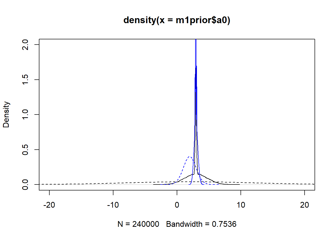

#showing density plots for b0
plot(density(m1prior$b0), xlim = c (-20,20), ylim = c(0,2), lty=2)
lines(density(m1post$b0), lty=1)
lines(density(m3prior$b0), col = "blue", lty=2)
lines(density(m3post$b0), col = "blue", lty=1)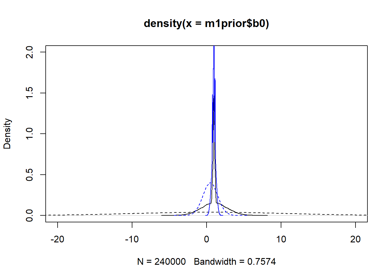

#showing density plots for a1
plot(density(m1prior$a1), xlim = c (-3,3), ylim = c(0,2), lty=2)
lines(density(m1post$a1), lty=1)
lines(density(m3prior$a1), col = "blue", lty=2)
lines(density(m3post$a1), col = "blue", lty=1)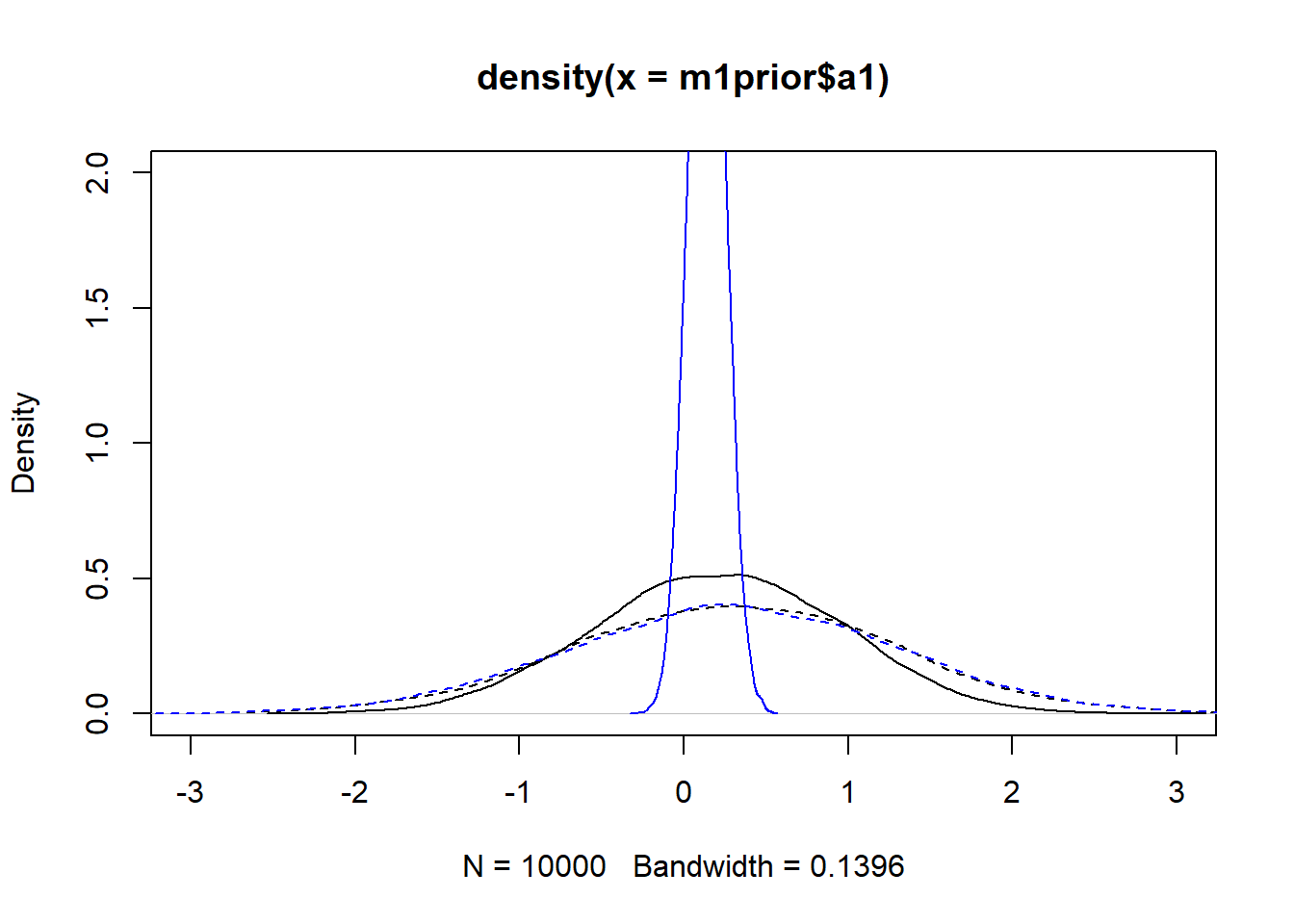

#showing density plots for b1
plot(density(m1prior$b1), xlim = c (-3,3), ylim = c(0,2), lty=2)
lines(density(m1post$b1), lty=1)
lines(density(m3prior$b1), col = "blue", lty=2)
lines(density(m3post$b1), col = "blue", lty=1)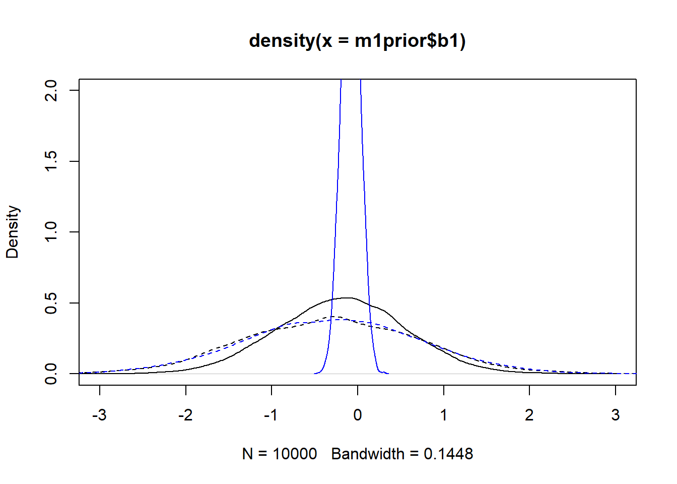

We set up the models to have wider $a_{0}$ and $b_{0}$ priors for model 1, and the same priors for the $a_{1}$ and $b_{1}$ parameters. The dashed lines in the figures show that. Looking at the posteriors, we find that changing the priors has an impact, especially for $a_{1}$ and $b_{1}$ . Not only does model 3 lead to more peaked posteriors, they are also not centered at the same values, especially for $b_{1}$ . I don’t think that’s a good sign. We want the data to dominate the results, the priors should just be there to ensure the models explore the right parameter space efficiently and don’t do anything crazy. The fact that the same model, started with different priors, leads to different posterior distributions is in my opinion concerning. It could be that with more sampling, the posteriors might get closer. Or it might suggest that we are overfitting and have non-identifiability problems here.

One way to check that further is to look at potential correlations between parameter posterior distributions, e.g., using a pairs() plot as shown above. Here are such plots for the parameters associated with $α$ for model 1. I only plot a few for each dose, otherwise the plots won’t be legible inside this html document. But you can try for yourself, if you make the plot large enough you can fit them all. You can also make plots for model 3 and for the $b$ parameters, those look very similar.

# all "a" parameters - too big to show
#pairs(fl[[1]]$fit, pars = c("a0","a1"))
# a few parameters for each dose
#low dose
rethinking::pairs(fl[[1]]$fit, pars = c("a0[1]","a0[2]","a0[3]","a0[4]","a1"))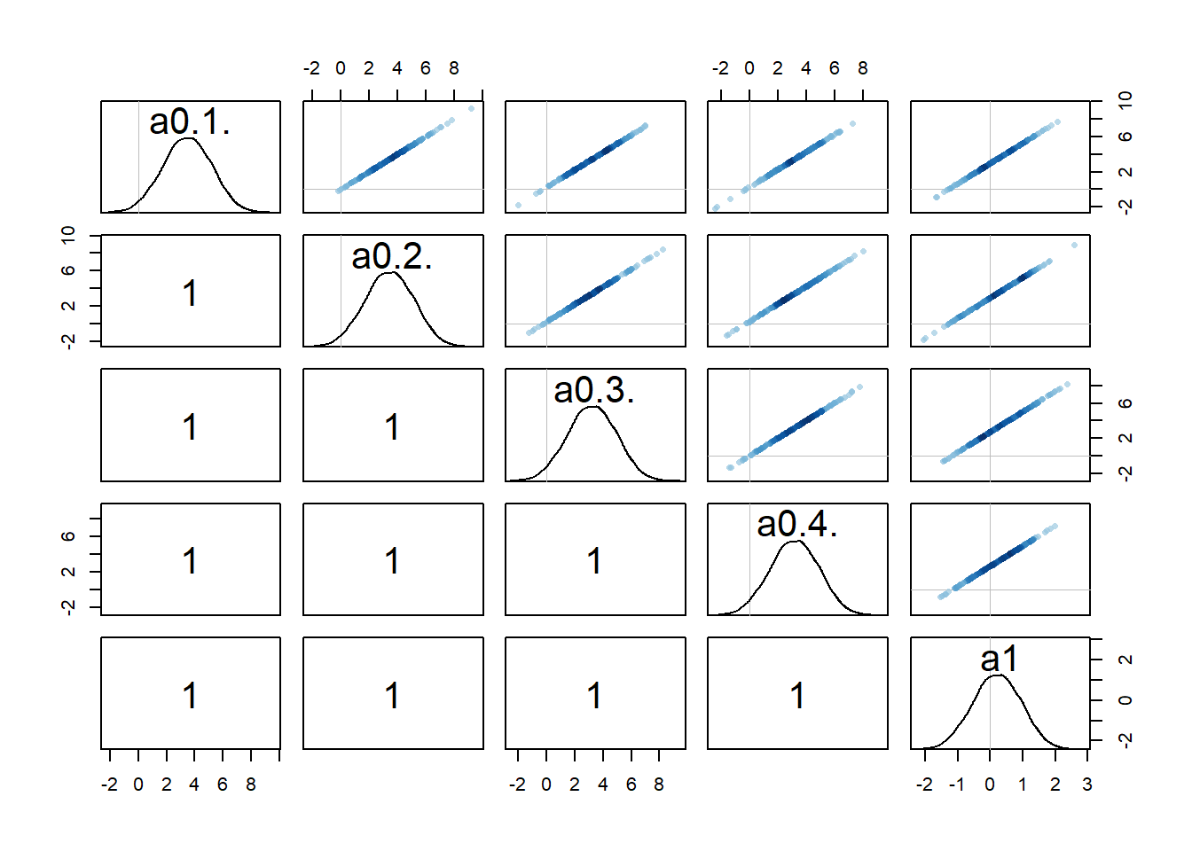

#medium dose
rethinking::pairs(fl[[1]]$fit, pars = c("a0[8]","a0[9]","a0[10]","a0[11]","a1"))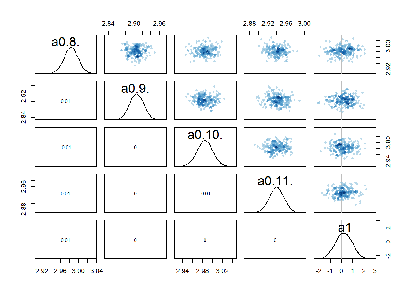

#high dose
rethinking::pairs(fl[[1]]$fit, pars = c("a0[16]","a0[17]","a0[18]","a0[19]","a1"))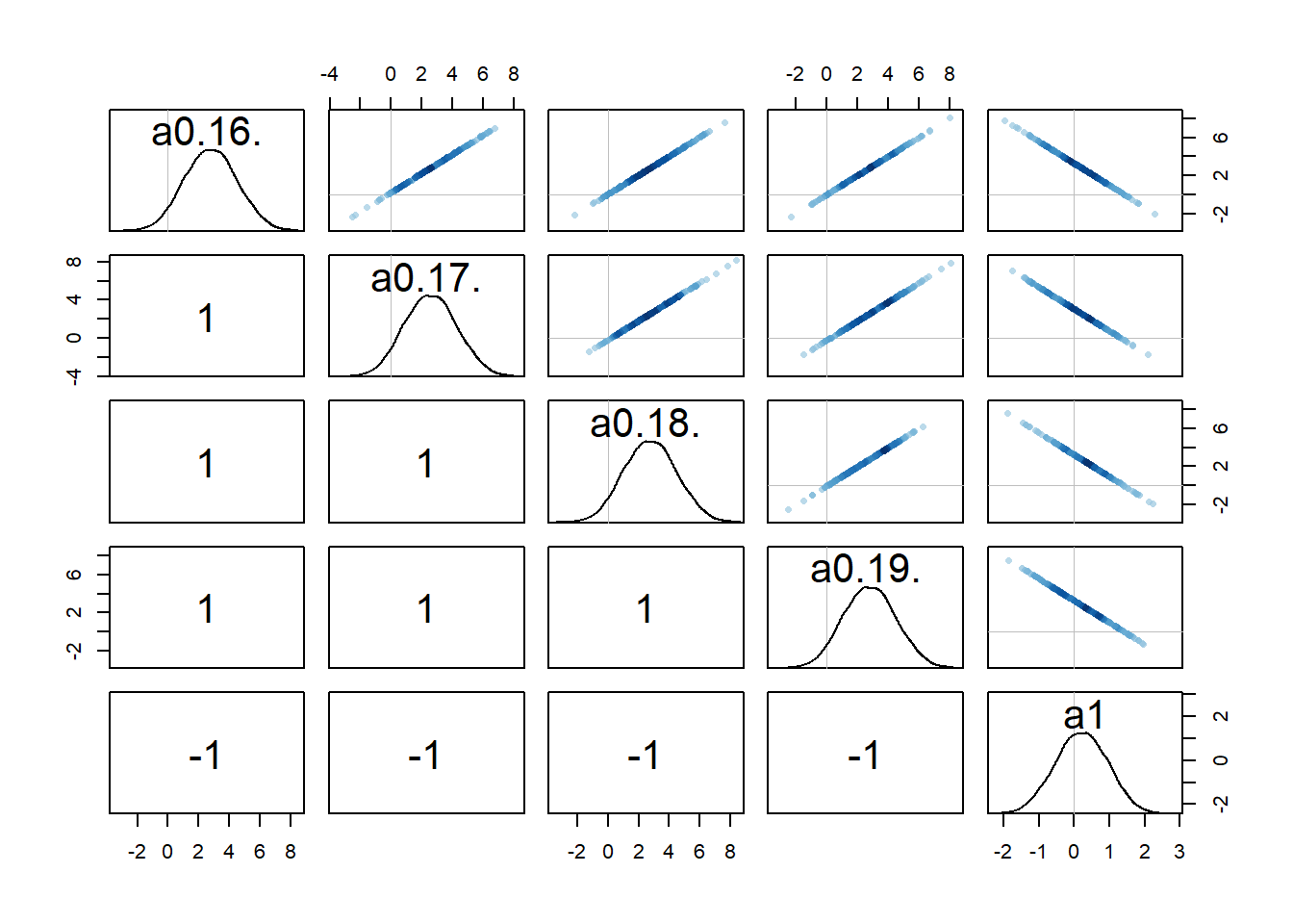

Recall that we set up the model such that dose is non-zero for low and high dose, while for the intermediate dose it drops out of the model. What seems to happen is that if the dose effect, i.e., $a_{1}$ , is present, there is a strong correlation among that parameter and the individual-level parameters for that dose. That part makes some sense to me. Both $a_{0, i}$ or $a_{1}$ can change $α$ and thus the trajectory. If one is low, the other might be high, and the reverse, leading to similarly good fits.

Because every $a_{0, i}$ is correlated with $a_{1}$ in this way, this also leads to correlations among the $a_{0, i}$ values. I am surprised that this is an essentially perfect correlation. Maybe, if I thought about it harder and/or did the math, it would be clear that it needs to be that way. But I haven’t yet, so for now I’m just taking it as given 😁. Overall, this is another sign of that we might be overfitting and have non-identifiability problems, i.e. combinations for different values of $a_{0, i}$ and $a_{1}$ can lead to more or less the same results (everything I write here of course also holds for the $b_{0, i}$ and $b_{1}$ parameters).

Let’s move on and now look at the posterior distributions in numerical form. For that, I use the precis function from rethinking. Instead of printing all the $N$ different values of $a_{0, i}$ and $b_{0, i}$ , I compute their means. If you want to see them all, change to depth=2 in the precis function.

# Model 1
a0mean = mean(rethinking::precis(fl[[1]]$fit,depth=2,"a0")$mean)
b0mean = mean(rethinking::precis(fl[[1]]$fit,depth=2,"b0")$mean)
print(rethinking::precis(fl[[1]]$fit,depth=1),digits = 2)

       mean    sd  5.5% 94.5% n_eff Rhat4
a1     0.20 0.743 -1.00  1.38  1359     1
b1    -0.19 0.744 -1.38  0.99  1120     1
sigma  1.06 0.051  0.99  1.15 10765     1

print(c(a0mean,b0mean))

[1] 2.963794 1.001530

# Model 3
a0mean = mean(rethinking::precis(fl[[3]]$fit,depth=2,"a0")$mean)
b0mean = mean(rethinking::precis(fl[[3]]$fit,depth=2,"b0")$mean)
print(rethinking::precis(fl[[3]]$fit,depth=1),digits = 2)

        mean    sd   5.5% 94.5% n_eff Rhat4
a1     0.142 0.109 -0.033 0.316  3298     1
b1    -0.081 0.107 -0.253 0.092  2648     1
sigma  1.061 0.051  0.983 1.146 13106     1

print(c(a0mean,b0mean))

[1] 2.9755846 0.9807953

The models seem to have converged ok, based on Rhat values of 1. Some parameters sampled better than others, as can be seen by the varying n_eff values. I used 5 chains of 2000 post-warmup samples for each chain, so the actual samples are 10000. If n_eff is lower than that, it means the sampling was not efficient, more means it worked very well (see e.g. Statistical Rethinking why it’s possible to get more effective samples than actual samples.)

We find that estimates for $a_{0}$ , $b_{0}$ and $σ$ are similar, $a_{1}$ and $b_{1}$ differ more.

Again, note that the only thing we changed between models 1 and 3 are to make the priors for the $a_{0, i}$ and $b_{0, i}$ parameters tighter. It didn’t seem to impact estimates for those parameters, but it did impact the estimates for the posterior distributions of parameters $a_{1}$ and $b_{1}$ . The numbers are consistent with the posterior distribution figures above.

Comparing model estimates with the truth

We know the “truth” here, i.e., the actual values of the parameters which we used to created the simulated data. To generate the data, we used these parameter values: $σ =$ 1, $μ_{a} =$ 3, $μ_{b} =$ 1, $a_{1} =$ 0.1, $b_{1} =$ -0.1. We also said that our main scientific question is if there is a dose effect, i.e. non-zero $a_{1}$ and $b_{1}$ .

The models find estimates of $μ_{a}$ , $μ_{b}$ and $σ$ that are close to what we used. The estimates for $a_{1}$ and $b_{1}$ are not that great. That’s especially true for model 1. With these models, we aren’t able to convincingly recover the parameters used to generate the data. I’m not sure if increasing the sampling (longer or more chains) would help. Both models, especially model 1, already took quite a while to run. Thus I’m not too keen to try it with even more samples. As we’ll see below, alternative models do better.

Models 2 and 2a

Next, let’s look at models 2 and 2a. The estimates should be similar since the two models are conceptually pretty much the same.

# Compare models 2 and 2a
# first we compute the mean across individuals for model 2
a0mean = mean(rethinking::precis(fl[[2]]$fit,depth=2,"a0")$mean)
b0mean = mean(rethinking::precis(fl[[2]]$fit,depth=2,"b0")$mean)

#rest of model 2
print(rethinking::precis(fl[[2]]$fit,depth=1),digits = 2)

        mean     sd  5.5%  94.5% n_eff Rhat4
mu_a   2.982 0.0221  2.95  3.020    34   1.1
mu_b   0.991 0.0191  0.96  1.023    30   1.2
a1     0.096 0.0097  0.08  0.110    87   1.0
b1    -0.097 0.0080 -0.11 -0.085   165   1.0
sigma  6.825 0.3217  6.35  7.334    50   1.1

print(c(a0mean,b0mean))

[1] 2.9823079 0.9908912

#model 2a
print(rethinking::precis(fl[[5]]$fit,depth=1),digits = 2)

        mean     sd  5.5%  94.5% n_eff Rhat4
a0     2.919 0.0237  2.88  2.955  5827     1
b0     0.938 0.0208  0.90  0.970  5976     1
a1     0.108 0.0108  0.09  0.125  6119     1
b1    -0.098 0.0096 -0.11 -0.083  6474     1
sigma  7.007 0.3188  6.51  7.542  7481     1

The first thing to note is that model 2 performs awfully, with Rhat values >1 and very low effective sample size n_eff. This indicates that this model doesn’t work well for the data. Whenever you see diagnostics like that, you should not take the estimated values seriously. However, let’s pretend for a moment that we can take them seriously. Here is what we find.

First, both models produce similar estimates. Since model 2a is simpler and doesn’t have that strange feature of us enforcing a very tight distribution for the $a_{0, i}$ and $b_{0, i}$ parameters, it actually samples much better, see the higher n_eff numbers. It also runs much faster, 1.6 minutes compared to 29 minutes for model 2.

Both models do a very poor job estimating $σ$ . That’s because we don’t allow the models to have the flexibility needed to fit the data, so it has to account for any variation between its estimated mean trajectory and the real data by making $σ$ large.

Since the models are more constrained compared to models 1 and 3, they produce estimates for $a_{1}$ and $b_{1}$ that are tighter. However, these estimates are over-confident. Overall these models are underfitting and not reliable. We can for instance look at this using the compare function:

rethinking::compare(fl[[1]]$fit,fl[[3]]$fit,fl[[2]]$fit,fl[[5]]$fit)

                 WAIC       SE       dWAIC        dSE    pWAIC        weight
fl[[3]]$fit  832.3041 23.37289   0.0000000         NA 43.47114  5.465565e-01
fl[[1]]$fit  832.6776 23.35188   0.3735338  0.3659438 43.55465  4.534435e-01
fl[[2]]$fit 1779.6905 45.62606 947.3863988 46.8519545 11.11914 1.035839e-206
fl[[5]]$fit 1788.5509 45.32354 956.2468479 47.0719252 10.52777 1.233873e-208

I’m not going to discuss things in detail (see Statistical Rethinking), but a lower WAIC means a model that fits best in the sense that it strikes a good balance between fitting the data while not overfitting. As you can see, models 1 and 3 perform very similarly and models 2 and 2a are much worse.

The larger WAIC indicates either strong overfitting or underfitting. In this case, it’s underfitting. The models are not flexible enough to capture the individual-level variation. You’ll see that clearly in the plots shown further below. If we did indeed not want to account for individual-level variation, we should go with a model that simply doesn’t include it, i.e. model 2a. The contrived model 2 with very narrow priors is just a bad model, and I’m really only exploring it here for demonstration purposes.

Models 4 and 4a

Now we get to the models we really care about. When I set up the models, I suggested that model 4 was similar to models 1-3, but with priors adaptively chosen. That didn’t apply during data generation/simulation since in that step, we always need to manually choose values. But during the fitting/estimation, we should expect that model 4 chooses priors in a smart way, such that it is better than the models where we fixed the priors. Let’s see what model 4 produces. We also look at model 4a, which is exactly the same model, just rewritten to potentially make the numerical fitting routine more efficient.

Let’s start with prior and posterior plots.

#get priors and posteriors for models 4 and 4a
m4prior <- rethinking::extract.prior(fl[[4]]$fit, n = 1e4)
m4post <- rethinking::extract.samples(fl[[4]]$fit, n = 1e4)

m4aprior <- rethinking::extract.prior(fl[[6]]$fit, n = 1e4)
m4apost <- rethinking::extract.samples(fl[[6]]$fit, n = 1e4)

As before, the dashed lines show the priors, the solid the posteriors. Black is model 4, blue is model 4a.

#showing density plots for a0
plot(density(m4prior$mu_a), xlim = c (-10,10), ylim = c(0,2), lty=2)
lines(density(m4post$mu_a), lty=1)
lines(density(m4aprior$mu_a), col = "blue", lty=2)
lines(density(m4apost$mu_a), col = "blue", lty=1)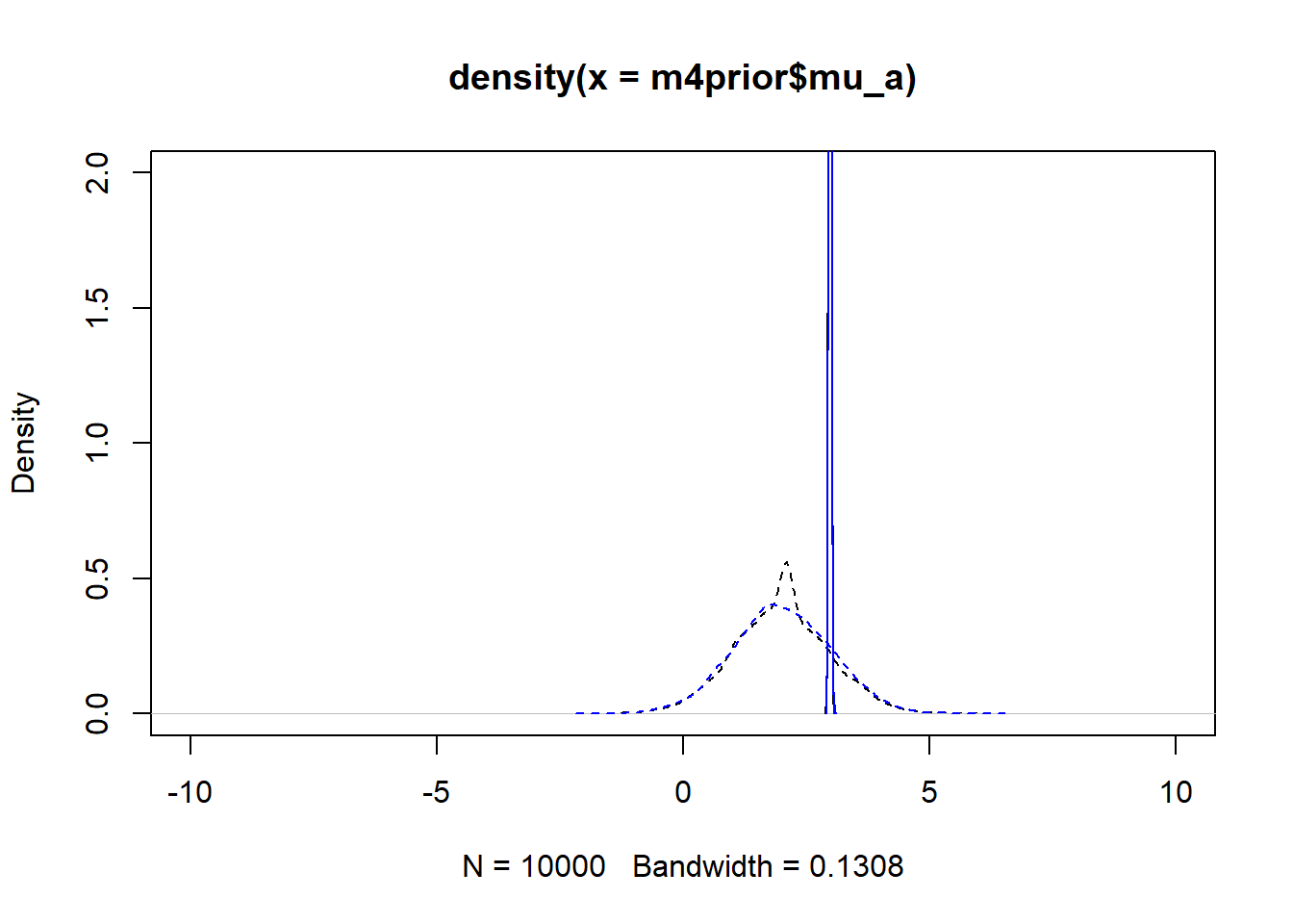

#showing density plots for b0
plot(density(m4prior$mu_b), xlim = c (-10,10), ylim = c(0,2), lty=2)
lines(density(m4post$mu_b), lty=1)
lines(density(m4aprior$mu_b), col = "blue", lty=2)
lines(density(m4apost$mu_b), col = "blue", lty=1)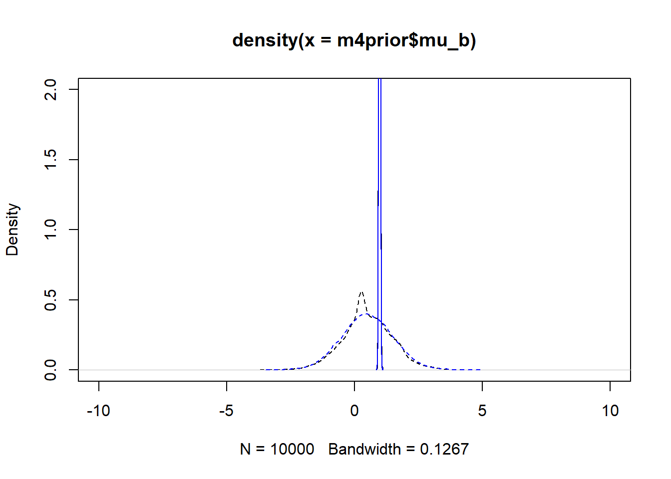

#showing density plots for a1
plot(density(m4prior$a1), xlim = c (-3,3), ylim = c(0,2), lty=2)
lines(density(m4post$a1), lty=1)
lines(density(m4aprior$a1), col = "blue", lty=2)
lines(density(m4apost$a1), col = "blue", lty=1)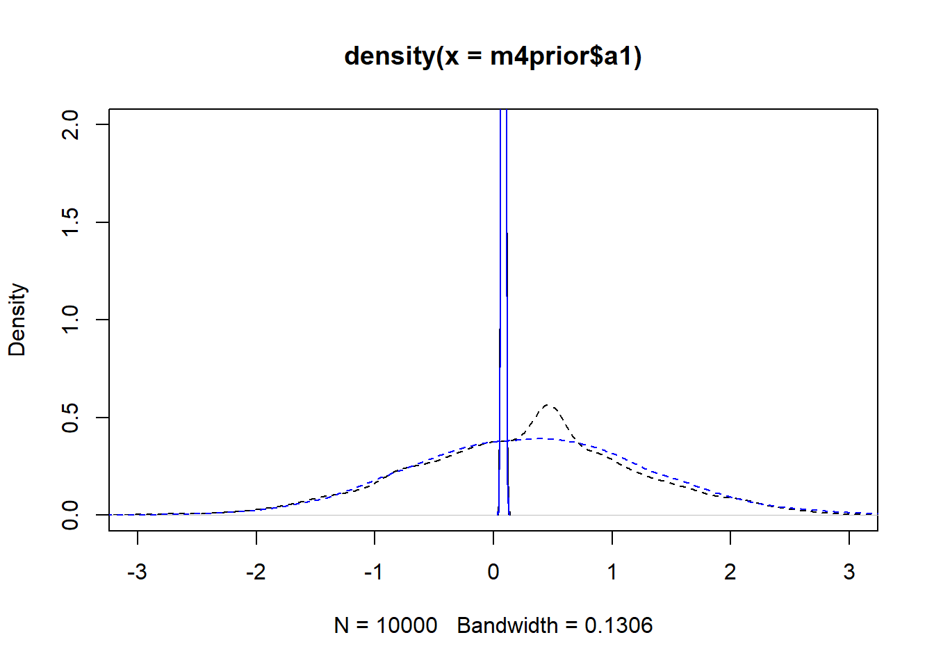

#showing density plots for b1
plot(density(m4prior$b1), xlim = c (-3,3), ylim = c(0,2), lty=2)
lines(density(m4post$b1), lty=1)
lines(density(m4aprior$b1), col = "blue", lty=2)
lines(density(m4apost$b1), col = "blue", lty=1)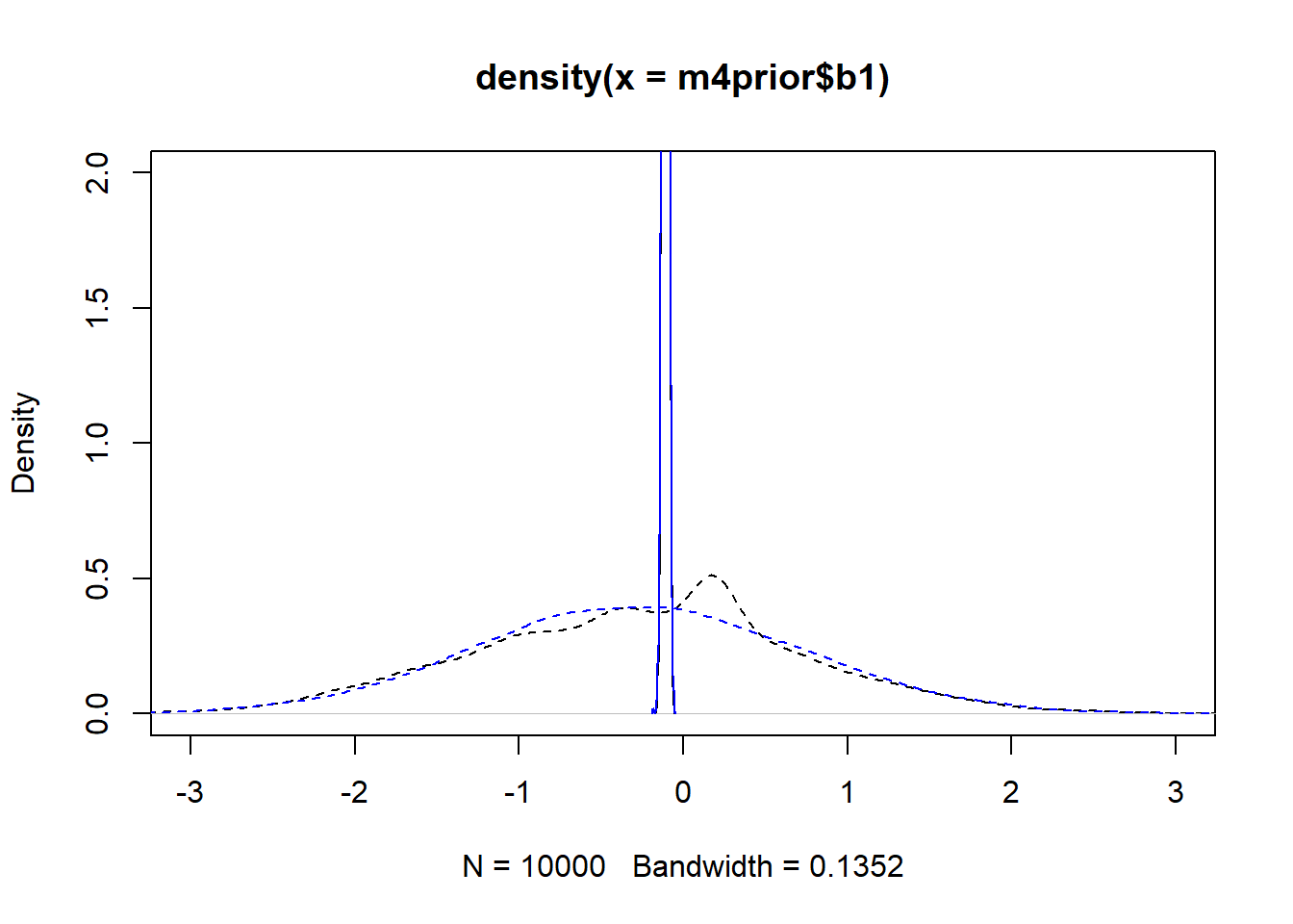

As you can see, up to numerical sampling variability, the results for models 4 and 4a are pretty much the same. That should be expected, since they are the same model, just reformulated for potential efficiency. Also, the posterior distributions are much narrower than the priors. I think that’s a good sign as well, it indicates the data mostly informed the posterior distributions, the priors just helped to keep things efficient.

We can also explore pair plots again, showing them here for model 4.

# a few parameters for each dose
#low dose
rethinking::pairs(fl[[4]]$fit, pars = c("a0[1]","a0[2]","a0[3]","a0[4]","a1"))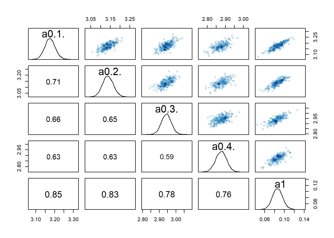

#medium dose
rethinking::pairs(fl[[4]]$fit, pars = c("a0[8]","a0[9]","a0[10]","a0[11]","a1"))

#high dose
rethinking::pairs(fl[[4]]$fit, pars = c("a0[16]","a0[17]","a0[18]","a0[19]","a1"))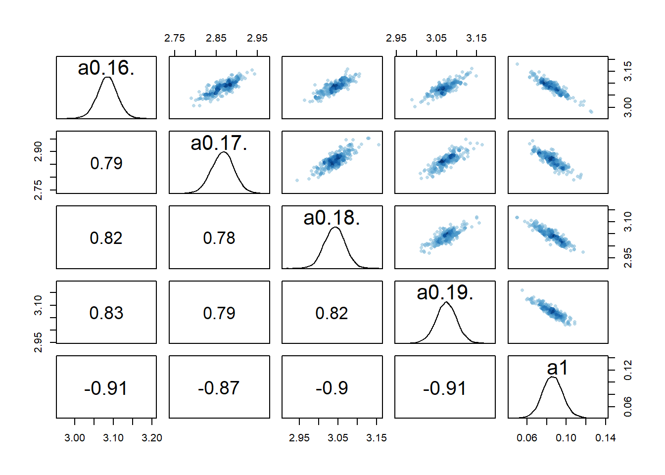

# mean of a0 prior
rethinking::pairs(fl[[4]]$fit, pars = c("mu_a","mu_b","a1","b1"))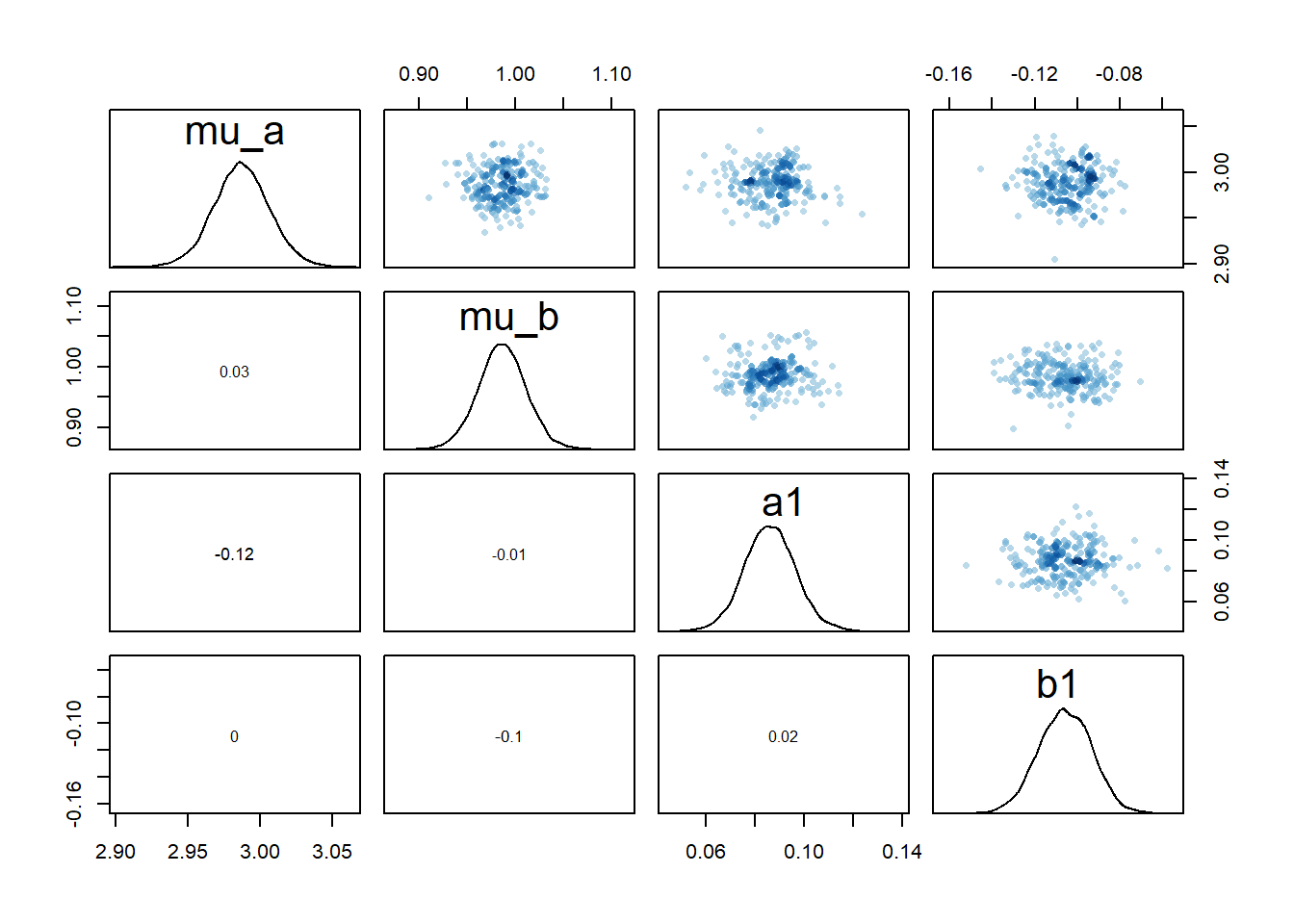

#saving one plot so I can use as featured image
png(filename = "featured.png", width = 6, height = 6, units = "in", res = 300)
rethinking::pairs(fl[[4]]$fit, pars = c("mu_a","mu_b","a1","b1"))
dev.off()

png 
  2

We still see the same issue with correlations among the parameters for dose levels where $a_{1}$ is acting, though the correlations are not as extreme. They are also minor between the overall estimates for the mean of the $a_{0}$ and $b_{0}$ parameters and $a_{1}$ and $b_{1}$ . I interpret this to mean that the adaptive sampling helped somewhat with the identifiability and overfitting problem, though it seems to not fully resolve it. The fact that we gave each individual their own $a_{0, i}$ and $b_{0, i}$ values allows those parameters to still “absorb” some of the dose-dependent signal in $a_{1}$ and $b_{1}$ .

We can also again look at the numerical outputs from the precis function.

# model 4
print(rethinking::precis(fl[[4]]$fit,depth=1),digits = 2)

          mean    sd   5.5%  94.5% n_eff Rhat4
mu_a     2.987 0.020  2.956  3.018 16421     1
mu_b     0.986 0.025  0.946  1.027 15631     1
sigma_a  0.093 0.015  0.072  0.120 11785     1
sigma_b  0.119 0.020  0.092  0.153 12447     1
a1       0.086 0.011  0.069  0.103  2057     1
b1      -0.106 0.013 -0.126 -0.086  2380     1
sigma    1.062 0.052  0.983  1.147 15009     1

# model 4a
print(precis(fl[[6]]$fit,depth=1),digits = 2)

          mean    sd   5.5%  94.5% n_eff Rhat4
mu_a     2.987 0.020  2.956  3.018  3254     1
mu_b     0.986 0.025  0.947  1.024  3029     1
sigma_a  0.093 0.016  0.071  0.120  3859     1
sigma_b  0.119 0.020  0.092  0.154  3542     1
a1       0.086 0.010  0.069  0.102  3771     1
b1      -0.106 0.013 -0.127 -0.085  3466     1
sigma    1.063 0.052  0.984  1.148  9032     1

The numerics confirm that the two models lead to essentially the same results. The values for n_eff differ between models, though neither model is consistently larger. This suggests that each model formulation had advantages in sampling for some of the parameters.

In terms of run times, there wasn’t much difference, with 6 minutes for model 4 versus 9 minutes for model 4a (much better than models 1-3).

If we compare the parameter estimates with the true values and those found for models 1 and 3 above, we find that again the true $μ_{a}$ , $μ_{b}$ and $σ$ are estimated fairly well. Estimates for $a_{1}$ and $b_{1}$ are now also pretty good, and the credible intervals are less wide.

Now let’s briefly run the compare function too and include model 3 as well. In addition to using WAIC for comparison, I’m also including PSIS. Read about it in the Statistical Rethinking book. One advantage of PSIS is that it gives warnings if the estimates might not be reliable. You see that this happens here.

rethinking::compare(fl[[3]]$fit,fl[[4]]$fit,fl[[6]]$fit, func = WAIC)

                WAIC       SE     dWAIC       dSE    pWAIC    weight
fl[[4]]$fit 831.3515 23.37623 0.0000000        NA 42.67688 0.4263132
fl[[6]]$fit 831.9958 23.38283 0.6442751 0.2846596 42.89029 0.3089059
fl[[3]]$fit 832.3041 23.37289 0.9525426 2.6103005 43.47114 0.2647810

#rethinking::compare(fl[[3]]$fit,fl[[4]]$fit,fl[[6]]$fit, func = PSIS)

We do find that model 4/4a performs a bit better, but not by much. Note that model 4/4a has more actual parameters, but the effective parameters (which is described by pWAIC) is a bit smaller.

Overall, this suggests that the adaptive pooling approach helped to estimate results more precisely and efficiently and is the best of the models.

Model 5

As stated above, due to a typo in my code, the above models, including 4/4a, initially produced estimates for $a_{1}$ and $b_{1}$ that were not close to those (I thought I) used to generate the data. Based on the pair plots, I suspected non-identifiability issues and wanted to explore what would happen if I removed the dose.

If we now look at the pairs plots, maybe not surprisingly, the correlations between individual $a_{0}$ parameters are gone.

# a few parameters for each dose
#low dose
rethinking::pairs(fl[[7]]$fit, pars = c("a0[1]","a0[2]","a0[3]","a0[4]","a0[5]"))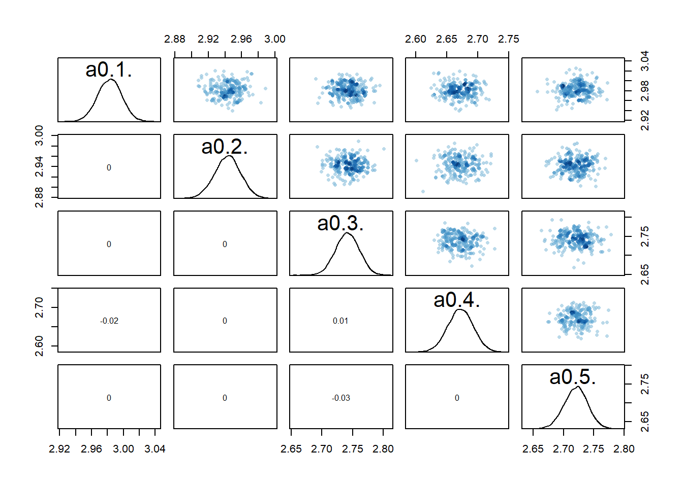

#medium dose
rethinking::pairs(fl[[7]]$fit, pars = c("a0[8]","a0[9]","a0[10]","a0[11]","a0[12]"))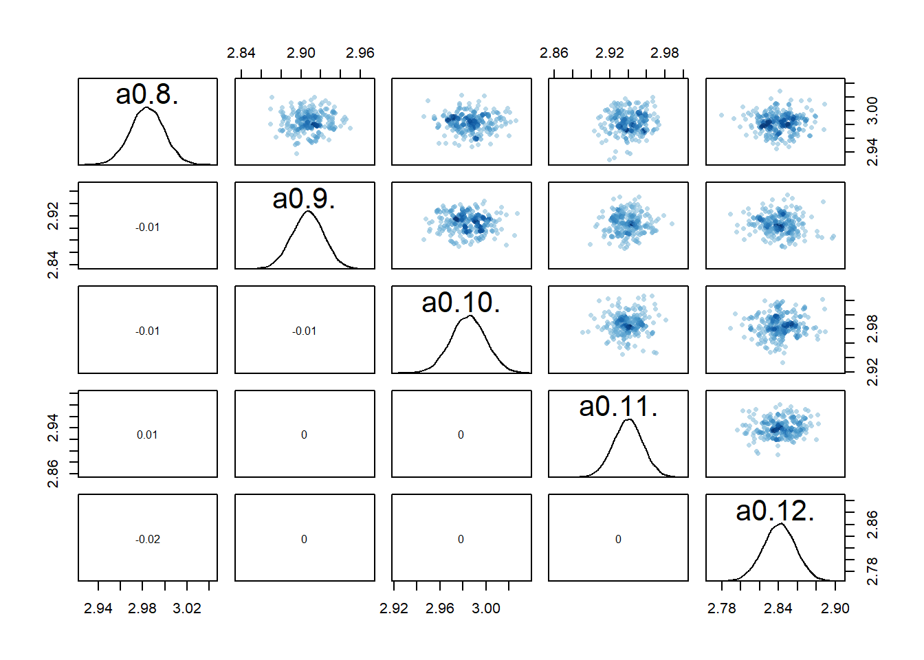

#high dose
rethinking::pairs(fl[[7]]$fit, pars = c("a0[16]","a0[17]","a0[18]","a0[19]","a0[20]"))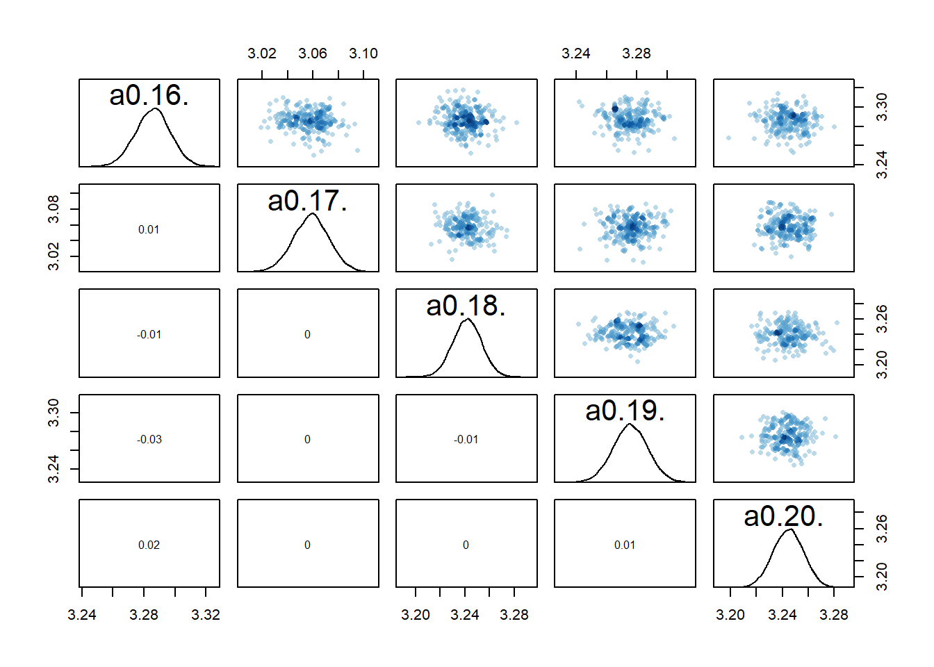

The model estimates the parameters reasonably well

a0mean = mean(rethinking::precis(fl[[7]]$fit,depth=2,"a0")$mean)
b0mean = mean(rethinking::precis(fl[[7]]$fit,depth=2,"b0")$mean)
print(rethinking::precis(fl[[7]]$fit,depth=1),digits = 2)

      mean    sd 5.5% 94.5% n_eff Rhat4
sigma  1.1 0.051 0.98   1.1 14886     1

print(c(a0mean,b0mean))

[1] 3.0031082 0.9655898

It doesn’t seem quite as good as the previous models.

rethinking::compare(fl[[3]]$fit,fl[[4]]$fit,fl[[7]]$fit)

                WAIC       SE     dWAIC      dSE    pWAIC    weight
fl[[4]]$fit 831.3515 23.37623 0.0000000       NA 42.67688 0.4462839
fl[[3]]$fit 832.3041 23.37289 0.9525426 2.610301 43.47114 0.2771847
fl[[7]]$fit 832.3088 23.33727 0.9572625 2.512509 43.43226 0.2765313

And of course the main problem with this model: It can’t answer any question about the role of dose, since we removed that component from the model! So while ok to explore, scientifically not useful since it can’t help us address the question we want to answer regarding the potential impact of dose.

Computing predictions

Looking at parameters as we did so far is useful. But we also want to see how model predictions look. It is possible to have a model that predicts overall well, even if the parameter estimates are not right (of course, for real, non-simulated data, we generally don’t know what the “right” values are). The opposite can’t happen, if you have the right model and the parameter estimates are right, the predictions will be good. But again, you never know if you have the right model, i.e., the model that captures the process underlying the data. For any real data, you almost certainly do not. Thus you could get parameters that look “right” (e.g. narrow credible intervals) but the model is still not good. Our models 2 and 2a fall into that category, as you’ll see below.

That is all to say, it’s important to look at model predicted outcomes, not just the parameters. So let’s plot the predictions implied by the fits for the models. The general strategy for that is to use the parameter estimates in the posterior, put them in the model, and compute the predictions. We are essentially going through the same steps we did to generate the data. Only now we start with the estimated values. While this could all be manually coded, we happily don’t need to do so. The rethinking package has some helper functions for that (sim and link).

The code below produces predictions, both for the deterministic mean trajectory $μ$ , and the actual outcome, $Y$ , which has added variation due to $σ$ .

#small data adjustment for plotting
plotdat <- fitdat %>% data.frame()  %>%
                      mutate(id = as.factor(id))  %>%
                      mutate(dose = dose_cat)

#this will contain all the predictions from the different models
fitpred = vector(mode = "list", length = length(fl))

# we are looping over each fitted model
for (n in 1:length(fl))
{
  #get current model
  nowmodel = fl[[n]]$fit

  #make new data for which we want predictions
  #specifically, more time points so the curves are smoother
  timevec = seq(from = 0.1, to = max(fitdat$time), length=100)
  Nind = max(fitdat$id)
  #new data used for predictions
  preddat = data.frame( id = sort(rep(seq(1,Nind),length(timevec))),
                        time = rep(timevec,Nind),
                        dose_adj = 0
  )
  #add right dose information for each individual
  for (k in 1:Nind)
  {
    #dose for a given individual
    nowdose = unique(fitdat$dose_adj[fitdat$id == k])
    nowdose_cat = unique(fitdat$dose_cat[fitdat$id == k])
    #assign that dose
    #the categorical values are just for plotting
    preddat[(preddat$id == k),"dose_adj"] = nowdose
    preddat[(preddat$id == k),"dose_cat"] = nowdose_cat
  }

  # pull out posterior samples for the parameters
  post <- rethinking::extract.samples(nowmodel)

  # estimate and CI for parameter variation
  # this uses the link function from rethinking
  # we ask for predictions for the new data generated above
  linkmod <- rethinking::link(nowmodel, data = preddat)

  #computing mean and various credibility intervals
  #these choices are inspired by the Statistical Rethinking book
  #and purposefully do not include 95%
  #to minimize thoughts of statistical significance
  #significance is not applicable here since we are doing bayesian fitting
  modmean <- apply( linkmod$mu , 2 , mean )
  modPI79 <- apply( linkmod$mu , 2 , PI , prob=0.79 )
  modPI89 <- apply( linkmod$mu , 2 , PI , prob=0.89 )
  modPI97 <- apply( linkmod$mu , 2 , PI , prob=0.97 )

  # estimate and CI for prediction intervals
  # this uses the sim function from rethinking
  # the predictions factor in additional uncertainty around the mean (mu)
  # as indicated by sigma
  simmod <- rethinking::sim(nowmodel, data = preddat)

  # mean and credible intervals for outcome predictions
  # modmeansim should agree with above modmean values
  modmeansim <- apply( simmod , 2 , mean )
  modPIsim <- apply( simmod , 2 , PI , prob=0.89 )

  #place all predictions into a data frame
  #and store in a list for each model
  fitpred[[n]] = data.frame(id = as.factor(preddat$id),
                            dose = as.factor(preddat$dose_cat),
                            predtime = preddat$time,
                            Estimate = modmean,
                            Q79lo = modPI79[1,], Q79hi = modPI79[2,],
                            Q89lo = modPI89[1,], Q89hi = modPI89[2,],
                            Q97lo = modPI97[1,], Q97hi = modPI97[2,],
                            Qsimlo=modPIsim[1,], Qsimhi=modPIsim[2,]
                            )
} #end loop over all models

Creating plots of the results

Now that we got the predictions computed, we can plot them and compare to the data. It turns out that trying to plot all the different credible intervals makes the plot too busy, so I’m only showing a few. You can play around by turning the commented lines on.

#list for storing all plots
plotlist = vector(mode = "list", length = length(fl))

#looping over all models, creating and storing a plot for each
for (n in 1:length(fl))
{
  #adding titles to plots
  title = fl[[n]]$model

  plotlist[[n]] <- ggplot(data = fitpred[[n]], aes(x = predtime, y = Estimate, group = id, color = dose ) ) +
    geom_line() +
    #geom_ribbon( aes(x=time, ymin=Q79lo, ymax=Q79hi, fill = dose), alpha=0.6, show.legend = F) +
    geom_ribbon(aes(x=predtime, ymin=Q89lo, ymax=Q89hi, fill = dose, color = NULL), alpha=0.3, show.legend = F) +
    #geom_ribbon(aes(x=time, ymin=Q97lo, ymax=Q97hi, fill = dose), alpha=0.2, show.legend = F) +
    geom_ribbon(aes(x=predtime, ymin=Qsimlo, ymax=Qsimhi, fill = dose, color = NULL), alpha=0.1, show.legend = F) +
    geom_point(data = plotdat, aes(x = time, y = outcome, group = id, color = dose), shape = 1, size = 2, stroke = 2) +
    scale_y_continuous(limits = c(-30,50)) +
    labs(y = "Virus load",
         x = "days post infection") +
    theme_minimal() +
    ggtitle(title)
}

Showing the plots

Here are the plots for all models we considered. I’m plotting them in the order I discussed the models above, so the ones we compared above are shown right below each other.

It’s a bit hard to see, but each plot contains for each individual the data as symbols, the estimated mean as line, and the 89% credible interval and prediction interval as shaded areas. The prediction interval is the light shaded area. If you enlarge the images, you should be able to see it.

Models 1 and 3

plot(plotlist[[1]])

plot(plotlist[[3]])

Despite differences in estimates for the dose related parameters, the predicted outcomes of the models are very similar. In fact, it’s hard to tell any difference by just looking at the plots (but they are slightly different, I checked). Thus, despite the inability of these models to provide precises estimates of all the parameter values, the predictions/outcomes are fine, they fit the data well.

Models 2 and 2a

For models 2 and 2a, recall that the only variation is for dose, we didn’t allow variation among individuals. That’s reflected in the plots. The credible intervals based on parameters are tight, but because the variability, $σ$ , had to account for all the differences, the prediction intervals are very wide.

plot(plotlist[[2]])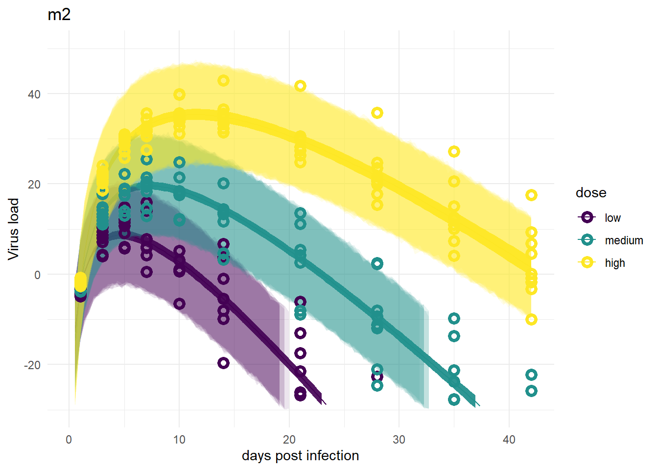

plot(plotlist[[5]])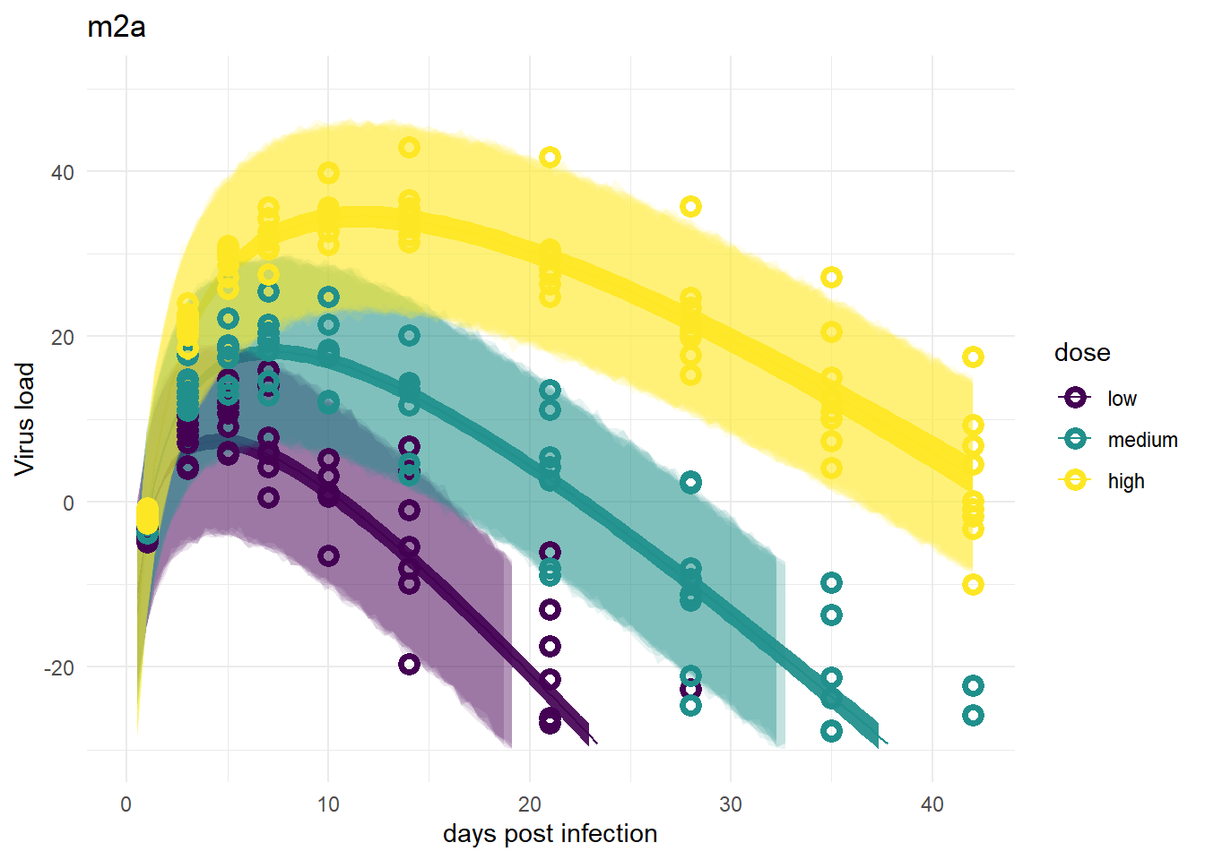

Models 4 and 4a

These models look good again, and very similar to models 1 and 3.

plot(plotlist[[4]])

plot(plotlist[[6]])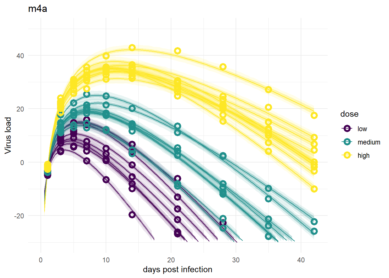

Model 5

The model fits look fine, suggesting that one parameter for each individual is enough to capture the data. That’s not surprising. However, this of course does not allow us to ask and answer any scientific questions about the role of dose.

plot(plotlist[[7]])

So overall, the figures make sense. It seems that if we want to do prediction, all models that include individual variability are fine, models 2/2a are not great. If we wanted to estimate the model parameters, specifically $a_{1}$ and $b_{1}$ , models 1 and 3 and of course 5 don’t work. In that case, model 2/2a works ok. I consider model 4/4a the best one overall.

For another example and more discussion of estimation versus prediction, see e.g. Section 6.1. in Statistical Rethinking, as well as 9.5.4 (all referring to the 2nd edition of the book).

Summary and continuation

To sum it up, we fit several models to the simulated time-series data to explore how different model formulations might or might not impact results. For this post, I used the - very nice! - rethinking package. In the next post, I’ll repeat the fitting again, now using brms. Since brms is very widely used and has some capabilities that go beyond what rethinking can do, I think it’s worth reading the next post.

If you don’t care about brms, you can hop to this post, where I discuss a few further topics and variations. Any fitting done in that post is with ulam/rethinking, so you don’t need to look at the brms post, but I still suggest you do 😁.

Footnotes

Note that I made the unfortunate choice of assigning the previously generated data to fitdat, which is not the same as the fitdat object I created in the Data Loading section above. I just noticed that a good while after I had written it all. So I won’t change it, but it would have been better if I had called it something different.↩︎